")
")
| Issue |
BSGF - Earth Sci. Bull.
Volume 190, 2019
|
|
|---|---|---|
| Article Number | 7 | |
| Number of page(s) | 15 | |
| DOI | https://doi.org/10.1051/bsgf/2019008 | |
| Published online | 14 June 2019 | |
Predicting the phase behavior of hydrogen in NaCl brines by molecular simulation for geological applications
Prédiction par simulation moléculaire des équilibres de phase de l’hydrogène dans des saumures de NaCl pour des applications géologiques
1
IFP Energies nouvelles,
1 et 4 avenue de Bois-Préau,
92852
Rueil-Malmaison, France
2
ENGIE,
1 Place Samuel de Champlain,
92400
Courbevoie, France
3
E2S UPPA, LCFR,
rue de l’Université,
64100
Pau, France
* Corresponding author: This email address is being protected from spambots. You need JavaScript enabled to view it.
Received:
14
January
2019
Accepted:
5
May
2019
Abstract
Hydrogen is targeted to have a significant influence on the energy mix in the upcoming years. Its underground injection is an efficient solution for large-scale and long-term storage. Furthermore, natural hydrogen emissions have been proven in several locations of the world, and the potential underground accumulations constitute exciting carbon-free energy sources. In this context, comprehensive models are necessary to better constrain hydrogen behavior in geological formations. In particular, solubility in brines is a key-parameter, as it directly impacts hydrogen reactivity and migration in porous media. In this work, Monte Carlo simulations have been carried out to generate new simulated data of hydrogen solubility in aqueous NaCl solutions in temperature and salinity ranges of interest for geological applications, and for which no experimental data are currently available. For these simulations, molecular models have been selected for hydrogen, water and Na+ and Cl− to reproduce phase properties of pure components and brine densities. To model solvent-solutes and solutes-solutes interactions, it was shown that the Lorentz-Berthelot mixing rules with a constant interaction binary parameter are the most appropriate to reproduce the experimental hydrogen Henry constants in salted water. With this force field, simulation results match measured solubilities with an average deviation of 6%. Additionally, simulation reproduced the expected behaviors of the H2O + H2 + NaCl system, such as the salting-out effect, a minimum hydrogen solubility close to 57 °C, and a decrease of the Henry constant with increasing temperature. The force field was then used in extrapolation to determine hydrogen Henry constants for temperatures up to 300 °C and salinities up to 2 mol/kgH2O. Using the experimental measures and these new simulated data generated by molecular simulation, a binary interaction parameter of the Soreide and Whiston equation of state has been fitted. The obtained model allows fast and reliable phase equilibrium calculations, and it was applied to illustrative cases relevant for hydrogen geological storage or H2 natural emissions.
Résumé
Dans les années à venir, l’hydrogène est amené à occuper une place toujours plus importante dans le mix énergétique. Son injection dans le sous-sol s’avère être une solution efficace pour son stockage à grande échelle et sur le long-terme. Par ailleurs, des émissions naturelles d’hydrogène ont été mises en évidence en plusieurs endroit du monde, et les accumulations souterraines potentielles constituent une source d’énergie décarbonée prometteuse. Dans ce contexte, des modèles sont nécessaires pour mieux appréhender le comportement de l’hydrogène dans les formations géologiques. En particulier, sa solubilité dans les saumures est un paramètre-clé, qui influence directement la réactivité de l’hydrogène et sa mobilité dans les milieux poreux. Dans ce travail, des simulations Monte Carlo ont été réalisées pour générer de nouvelles données simulées de solubilité d’hydrogène dans des solutions aqueuses de NaCl pour des gammes de températures et pressions représentatives des conditions géologiques, et pour lesquelles aucune donnée expérimentale n’est aujourd’hui disponible. Pour ces simulations, des modèles moléculaires existants ont été sélectionnés pour l’hydrogène, l’eau et les ions Na+ et Cl− afin de reproduire les propriétés des corps purs et les densités de la saumure. Pour modéliser les interactions solvant-soluté et soluté-soluté, nous avons montré que les règles de mélange de Lorentz-Berthelot avec un paramètre d’interaction binaire constant sont les plus appropriées pour reproduire les données expérimentales disponibles de constante de Henry de l’hydrogène dans l’eau salée. Avec ce champ de forces, les résultats de simulation reproduisent les données expérimentales de solubilité avec un écart moyen de 6 %. De plus, les simulations reproduisent les comportements attendus du système H2 + H2O + NaCl, comme l’effet « salting-out », le minimum de solubilité vers 57 °C et la diminution de la constante de Henry lorsque la température augmente. Ce champ de forces a alors été utilisé en extrapolation pour déterminer les constantes de Henry de l’hydrogène pour des températures jusqu’à 300 °C et des salinités jusqu’à 2 mol/kgH2O. En utilisant les données expérimentales existantes et ces nouvelles données simulées générées par la simulation moléculaire, un coefficient d’interaction binaire a été ajusté pour l’équation d’état Soreide et Whitson. Le modèle ainsi construit permet des calculs rapides et fiables des équilibres de phase impliquant l’hydrogène, et il a été appliqué sur des cas d’application représentatifs du stockage géologique et des émissions naturelles d’hydrogène.
Key words: hydrogen / solubility / Monte Carlo simulation / equation of state / H2 underground storage / H2 natural emissions
Mots clés : hydrogène / solubilité / simulation Monte Carlo / équation d’état / stockage souterrain de l&apos / hydrogène / émissions naturelles d’hydrogène
© C. Lopez-Lazaro et al., Published by EDP Sciences 2019
 This is an Open Access article distributed under the terms of the Creative Commons Attribution License (http://creativecommons.org/licenses/by/4.0), which permits unrestricted use, distribution, and reproduction in any medium, provided the original work is properly cited.
1 Introduction
Hydrogen (H2) is currently taking an increasing role in the energy mix. If hydrogen remains today a main raw material for the industry, its capacity for long-term storage of decarbonized energy is highlighted by numerous authors and the H2 council. First pilot projects are taking place and use electrolyzers to convert solar- and wind-farm electricity to H2 which is then stored (Darras et al., 2012; Perez et al., 2016). It can then be converted again to electricity (such as the Methycentre project [ADEME, 2018]), injected in the natural gas network (such as the Grhyd project in Dunkerque, France [ENGIE, 2018]) or used as fuel for vehicles. But the development of a large-scale use of hydrogen implies increasing storage needs, and injection in geological formations, used extensively in the gas and compressed air energy industries, is an attractive solution to reach sizable storage volumes (Lord et al., 2014). Various options that already proved their efficiency and economic viability for other gases, such as injection in aquifers, depleted oil and gas fields, and salt caverns, are currently under study (Le Duigou et al., 2017).
In addition, numerous native H2 emissions have been detected worldwide, in the mid oceanic ridge, in active fault zones, in ophiolitic contexts or in intracratonic basins (Charlou et al., 2002; Charlou et al., 2010; Deville and Prinzhofer 2016; Larin et al., 2015; Moretti et al., 2018; Prinzhofer and Deville, 2015; Satake et al., 1984; Sato et al., 1986; Vacquand et al., 2018). Accumulations have even been found in Kansas (Guélard et al., 2017) or Mali (Prinzhofer et al., 2018), where natural hydrogen is used to produce electricity since 2015. The sources of H2 and the mechanisms responsible for its formation remain to be clearly identified, even if some chemical reactions are already known to be efficient H2 producers, such as serpentinization or oxidation of iron-rich rocks (Bachaud et al., 2017; Deville and Prinzhofer 2016; Vacquand et al., 2018). The behavior of this molecule along its migration path is another aspect that needs to be better constrained. The high mobility and reactivity of hydrogen have been highlighted in numerous studies (Carden and Paterson, 1979; Paterson, 1983; Reitenbach et al., 2015), both of which being impacted by hydrogen solubility in formation waters. Understanding the phase behavior of systems involving hydrogen and brines is thus of primary importance for exploration of native H2 accumulations and to correctly design hydrogen storage in geological formations.
Various equations of state have been already developed to accurately predict solubility of hydrogen in pure water at high temperature and pressure for geological applications (e.g. Akinfiev and Diamond, 2003; Plyasunov and Bazarkina, 2018; Plyasunov and Shock, 2001). Concerning electrolytic aqueous solutions, light gas solubility has been successfully modeled in the past using either activity coefficient models mainly based on the Pitzer theory (e.g. Duan and Sun, 2003; Duan et al., 1992; Li et al., 2018; Rumpf et al., 1998; Xia et al., 2000; Xia et al., 1999) or equations of state such as Virial-based equations (e.g. Duan et al., 1996, 2003), cubic equations (e.g. (Li et al., 2015; Soreide and Whitson, 1992; Sorensen et al., 2002), or more advanced equations of state including association forces as e-CPA (e.g. Carvalho et al., 2015; Courtial et al., 2014; Hemptinne et al., 2006; Kontogeorgis and Folas, 2010; Maribo-Mogensen et al., 2015) or e-SAFT (e.g. Ahmed et al., 2018; Held et al., 2014; Ji et al., 2005; Llovell et al., 2012; Patel et al., 2003; Rozmus et al., 2013; Sun and Dubessy, 2012). Nevertheless, all of these models involve empirical parameters to be fitted on available experimental data. Their application range is thus restricted to the temperature, pressure and salinity ranges of the experimental data used for their parameterization.
Concerning hydrogen solubility in brines, an important issue is the lack of experimental data in thermodynamic conditions relevant for geological applications. As described in the first section of this article, almost all the available solubility data concern temperature less than 303 K, and salinities less than 1 mol/kgH2O. The acquisition of new experimental data is a challenging and costly task for safety reasons (high flammability of hydrogen, corrosive aspect of brines) and technical aspects (low H2 solubility). In this context, a promising alternative is molecular simulation. Thanks to robust simulations, Monte Carlo simulation technique has become a very powerful method to predict thermodynamic data and phase equilibrium of systems of industrial interest (Theodorou, 2010; Ungerer et al., 2005). When using an appropriate force field, molecular simulation can be seen as a reliable tool to generate data in complement of classical experiments.
Previous studies have demonstrated the ability of Monte Carlo simulation to predict gas solubility in brines, such as CO2 (Creton et al., 2018; Jiang et al., 2017; Liu et al., 2013; Tsai et al., 2016; Vorholz et al., 2004), H2S (Fauve et al., 2017), SO2 and other diatomic light gases (Creton et al., 2018). However, to the best of our knowledge, no molecular simulation study dealing with the solubility of hydrogen in electrolyte solutions has been published. Hence, the goal of this work is first to validate a force field able to accurately predict hydrogen solubility in aqueous NaCl solutions over a wide range of temperatures and salt concentrations, and second to use the simulation data in complement of the existing experimental data to recalibrate an equation of state.
This paper is organized as follows: in a first section, a literature review is carried out to build a consistent database for H2 + H2O and H2 + H2O + NaCl systems. In a second section, a force field able to reproduce experimental data for both salt-free and salted systems is proposed. Then, Monte Carlo simulations are carried out at higher temperatures and salinities to generate new simulated data. In a third section, experimental and simulated solubility data are used to recalibrate the Soreide and Whitson equation of state (Soreide and Whitson, 1992) applicable over wide ranges of temperature, pressure and salinity. Finally, some geological applications for this new model are provided in the context of hydrogen storage and naturally-produced subsurface hydrogen. Today, underground gas storage as well as natural gas production refer mainly to hydrocarbon. As a comparison, we conclude on the difference between the methane and the H2 solubility and so transport and accumulation modes in subsurface.
2 Experimental data review
2.1 H2 + H2O system
A very large number of experimental data for hydrogen solubility in pure water is available in literature. Most of the data consist in volume ratio measurements, such as Bunsen, Kuenen and Ostwald coefficients. Some other data are also provided as direct measurement of solubility in mole fraction using PVT cells (“TPxy” data) or Henry constants. In order to easily compare data and build a consistent database, all these experimental data are converted in this work in term of Henry constant. Henry constant of a solute i is defined by:
 (1)
where xi and yi stands for mole fraction in liquid and vapor phase, respectively, fi the fugacity, P the total pressure and
(1)
where xi and yi stands for mole fraction in liquid and vapor phase, respectively, fi the fugacity, P the total pressure and  the fugacity coefficient in the vapor phase. If we assume the liquid concentration of the solute small enough, this equation becomes:
 (2)
(2)
Kuenen coefficient Si, Ostwald coefficients Li, and Bunsen coefficients αi are first converted in mole fraction xi using recommendations of the IUPAC guide (Gamsjäger et al., 2010):
 (3)
where Tθ and Pθ are standard temperature (273.15 K) and pressure (1.013 bar),
(3)
where Tθ and Pθ are standard temperature (273.15 K) and pressure (1.013 bar),  is the liquid molar volume of pure water and MS the molar mass of pure water.
Mole fractions are then converted in Henry constant using equation (2). The fugacity coefficient of hydrogen in vapor phase is calculated with the Soave-Redlich-Kwong equation of state (Soave, 1972) after having checked that this model is able to accurately reproduce pure hydrogen reference compressibility factors (Younglove, 1982). Solubility data (“TPxy” data) are also converted in Henry constants with equation (2) by taking for a given isotherm the smallest available experimental partial pressure to stay as close as possible of the infinite dilution domain. Finally, Table 1 details the type and the references of the various experimental data selected in this work for the binary system H2 + H2O. From these experimental data, the evolution of the Henry constant of H2 in pure water is shown on Figure 1. The repeatability of the experiments coming from various authors allows to evaluate an average experimental uncertainty of ±10%.
The experimental Henry constants are correlated using the formulation recommended by Trinh et al. for hydrogen Henry constant in oxygenated solvents (Trinh et al., 2016a):
 (4)
where Tr is the reduced temperature of water (Tr = T/Tc with Tc = 647.096 K),
(4)
where Tr is the reduced temperature of water (Tr = T/Tc with Tc = 647.096 K),  is the vapor pressure of pure water, and a, b, c are three adjustable parameters. The advantage of such an equation form is to allow extrapolation at high temperatures up to solvent critical temperature, as well as at low temperatures through the third term of the equation. The vapor pressure of pure water is evaluated from the DIPPR correlation (Rowley et al., 2003). The parameters a, b and c have been fitted to minimize the average absolute deviation (AAD) between the experimental and the correlated Henry constants. The optimized parameters are given in Table 2, and lead to an AAD of 4%, which is less than the experimental uncertainties. Thus, this correlation will be used further in this work to validate molecular simulation results. The correlation curve is plotted on Figure 1, and is valid from 273 K to 636 K.
Experimental data exhibit a maximum in the Henry constant curve for a temperature close to 330 K (i.e. about 57 °C), indicating that hydrogen solubility is minimal at this temperature. This is the typical behavior for the solubility of a small molecule in pure water, the minimum-solubility temperature depending on the nature of the solute (Ahmed et al., 2016).
Selected experimental data for H2 + H2O and H2 + H2O + NaCl systems.
 |
Fig. 1 Compilation of data: Henry constant of H2 in pure water versus temperature. Symbols: experimental data (circles: from Bunsen coefficients, diamonds: Henry constants, triangles: from TPx data, crosses: from Kuenen coefficients, stars: from Ostwald coefficients). Solid line: correlation (Eq. (3)). Dotted lines: uncertainty domain (±10% from the correlation). |
2.2 H2 + H2O + NaCl system
Some experimental data for hydrogen solubility in aqueous NaCl solutions are available in literature, but they concern very limited temperature and salinity ranges. All the data available are provided under Bunsen coefficient form, and have been converted into Henry constant as previously described. Note that in this conversion, the density of the solvent is required, and to this end the model of Rowe and Chou (Rowe, 1970) was used to calculate density of NaCl aqueous solution at the desired temperature and salt concentration. The most significant contribution is the work of Crozier and Yamamoto (1974) who acquired a large amount of hydrogen solubility data in seawater and NaCl aqueous solutions. Among the other data available, those of Braun (1900) have been rejected because they were found inconsistent with all other available data in similar conditions. Finally, a total of 296 consistent data are considered, and references are detailed in Table 1.
It is worth noticing that 95% of these data concern salt concentrations less than 1 mol/kgH2O (that is, 58 g/L, twice the usual salinity of seawater) and temperatures less than 303 K. As these operating conditions are very far from temperatures and even salinities that can be encountered in geological formations, it fully justifies the need to generate new data at higher temperature and salinity. Figure 2 shows a selection of Henry constants as a function of temperature for various salinity values. As data are mainly restricted to low temperatures, they cannot be correlated as previously done for pure water. Nevertheless some typical behaviors can be emphasized. First, the greater the molality, the greater the value of Henry constant. This is a consequence of the “salting-out” effect which corresponds to the solubility decrease when salt concentration in water increases. Second, as observed for pure water, data seem to exhibit a maximum in the curve comprised between 320 and 350 K.
 |
Fig. 2 Experimental and computed Henry constant of H2 in aqueous NaCl solutions versus temperature. Open symbols: experimental data. Filled symbols: simulation results with modified Lorentz-Berthelot combining rule and lij = 0.24 (diamonds: NaCl = 0.5 mol/kgH2O, squares: NaCl = 1 mol/kgH2O, triangles: NaCl = 2 mol/kgH2O). |
3 Monte Carlo simulation
3.1 Force field
The molecular model used for hydrogen is the model of Darkrim et al. (1999). This choice is motivated by a previous study led on hydrogen solubility in organic solvents (Ferrando and Ungerer, 2007) which showed that this molecular model is able to accurately reproduce pure hydrogen compressibility factor over a large temperature range and is particularly suitable for phase equilibrium calculation. The hydrogen molecule is represented by a single Lennard-Jones spheres with three point charges aim to mimic the quadrupole moment of the molecule. Details of this model are given in Table 3.
For aqueous NaCl solutions, the combination of the TIP4P/2005 model for pure water (Abascal and Vega, 2005) and the OPLS model for Na+ and Cl− (Chandrasekhar et al., 1984) is selected. The TIP4P/2005 model is able to accurately reproduce pure water density and vapor pressures, and it has been shown in a recent study (Creton et al., 2018) that its combination with the OPLS model for ions allows to reproduce correctly densities and osmotic pressures of aqueous NaCl solutions over a large temperature and salinity range. Details of these molecular models are given in Table 3.
In this work, all molecules are assumed rigid, and consequently only intermolecular interactions are taken into account. Intermolecular interactions are split into an electrostatic contribution and a Van der Waals dispersive-repulsive forces contribution. The dispersion-repulsion energy between two particles i and j is given by the Lennard-Jones potential:
 (5)
where rij is the distance between the two particles, and ϵij and σij the cross-energy and cross-diameter Lennard-Jones parameters, respectively. For both electrostatic and dispersive/repulsive interactions, a cut-off radius equal to the half of the simulation box is imposed. Ewald summation and classical tail correction (Allen and Tildesley, 1987) are employed to compute these interactions beyond the cut-off radius. To calculate the cross-energy and cross-diameter parameters for different type of molecules (e.g. H2 + H2O molecules), combining rules have to be chosen. The classical Lorentz-Berthelot combining rules (see Tab. 4) are used for water – Na+ and water – Cl− interactions. For water – hydrogen interactions, three usual combining rules are evaluated: Lorentz-Berthelot, Kong (Kong, 1973) and Waldmann-Hagler (Waldmann and Hagler, 1993). The choice of evaluating the two last combining rules is motivated by the fact that they led to accurate results for calculating phase equilibrium of other light gases in previous studies (Delhommelle and Millie, 2001; Ungerer et al., 2004). Finally, the combining rules selected for interactions between hydrogen and ions Na+ and Cl− are the rules of Lorentz-Berthelot, but as explained further in this work they have to be corrected by an interaction binary parameter.
(5)
where rij is the distance between the two particles, and ϵij and σij the cross-energy and cross-diameter Lennard-Jones parameters, respectively. For both electrostatic and dispersive/repulsive interactions, a cut-off radius equal to the half of the simulation box is imposed. Ewald summation and classical tail correction (Allen and Tildesley, 1987) are employed to compute these interactions beyond the cut-off radius. To calculate the cross-energy and cross-diameter parameters for different type of molecules (e.g. H2 + H2O molecules), combining rules have to be chosen. The classical Lorentz-Berthelot combining rules (see Tab. 4) are used for water – Na+ and water – Cl− interactions. For water – hydrogen interactions, three usual combining rules are evaluated: Lorentz-Berthelot, Kong (Kong, 1973) and Waldmann-Hagler (Waldmann and Hagler, 1993). The choice of evaluating the two last combining rules is motivated by the fact that they led to accurate results for calculating phase equilibrium of other light gases in previous studies (Delhommelle and Millie, 2001; Ungerer et al., 2004). Finally, the combining rules selected for interactions between hydrogen and ions Na+ and Cl− are the rules of Lorentz-Berthelot, but as explained further in this work they have to be corrected by an interaction binary parameter.
The electrostatic energy between two partial charges i and j is given by the Coulomb potential:
 (6)
where ϵ0 is the vacuum permittivity. The Ewald summation technique is employed to compute long-range corrections, with a Gaussian width α equal to 2 in reduced units and a number of reciprocal vectors k ranging from −7 to 7 in all three directions.
(6)
where ϵ0 is the vacuum permittivity. The Ewald summation technique is employed to compute long-range corrections, with a Gaussian width α equal to 2 in reduced units and a number of reciprocal vectors k ranging from −7 to 7 in all three directions.
Molecular models used in this work.
Combining rules evaluated for the H2O − H2 interactions.
3.2 Algorithm
The objective of the completed simulations is to compute the Henry constant of hydrogen in NaCl aqueous solutions, or in other words its chemical potential in liquid phase since at infinite dilution these two properties are linked by the relationship:
 (7)
where
(7)
where  and
and  are the fugacity and the chemical potential of i in the reference state, respectively, T is the temperature, R the ideal gas constant and xi the mole fraction of i in the liquid phase. The reference state can be chosen arbitrarily. In this work, the reference state corresponds to a zero chemical potential in a hypothetical pure ideal gas of unit density (1 molecule per Å3, i.e. a density
  mol/m3). In this reference state, the fugacity is equal to:
  . The excess chemical potential is defined by:
  .
.
Many methods exist to compute the excess chemical potential from molecular simulation. One of the most used is the so-called Widom particle insertion method (Frenkel and Smit, 1996; Widom, 1963). This method allows to compute excess chemical potential with a reasonable computation time in the NPT ensemble from:
 (8)
where kB is the Boltzmann constant, T the temperature, P the pressure, V the volume, N the number of molecules in the system and ΔU the energy difference related to the insertion of a solute molecule i.
(8)
where kB is the Boltzmann constant, T the temperature, P the pressure, V the volume, N the number of molecules in the system and ΔU the energy difference related to the insertion of a solute molecule i.
Aqueous NaCl solutions form a well-structured liquid phase in which the insertion move can be often rejected. Thus, Widom insertion method could appear in this context less efficient than more advanced techniques to evaluate chemical potential, such as umbrella sampling (Torrie and Valleau, 1977), slow-growth method (Nezbeda and Kolafa, 1991) or thermodynamic integration (Frenkel and Smit, 1996). Nevertheless, a prior study on the solubility of H2S in NaCl aqueous solution (Fauve et al., 2017) shown that, with a sufficient number of Monte Carlo steps, the Widom insertion method lead to similar results than thermodynamic integration technique within statistical uncertainties.
The Widom insertion method is applied during a Monte Carlo simulation in the NPT ensemble. This ensemble consists in one single box representing the liquid phase, where the total number of molecule N, the temperature T and the pressure P are imposed. For a given temperature, simulations are carried out at a pressure equal to the vapor pressure of the pure solvent (computed with the current force field). A total number of 500 molecules of water is used, and the number of Na+ and Cl− ions is chosen according to the desired molality (for example 9 particles of Na+ and Cl− for a molality of 1 mol/kgH2O). A simulation consists typically in an equilibrium run of about 200 to 500 million Monte Carlo steps to achieve equilibrium state, followed by a production run lasting for additional 400 million Monte Carlo steps to compute average properties. Each step generates a new configuration, which is accepted or rejected following the classical Metropolis criterion (Frenkel and Smit, 1996). The excess chemical potential value required in equation (8) is computed each 50 000 steps. The different Monte Carlo moves and their corresponding attempt probabilities used during a simulation are molecular translation (20%), molecular rotation (20%), insertion move (59.5%) with a pre-insertion statistical bias (Mackie et al., 1997) using 10 trial positions, and volume change (0.5%). The amplitude of translations, rigid rotations and volume changes was adjusted during the simulation to achieve an acceptance ratio of 40% for these moves. The simulations are carried out using the GIBBS software jointly developed by IFP Energies nouvelles and the Laboratoire de Chimie-Physique (CNRS-Université Paris-Sud) (Ungerer et al., 2005).
3.3 Results
3.3.1 System H2 + H2O
Monte Carlo simulation of the system H2 + H2O have been carried out with the three combining rules of Table 4 for the water – hydrogen cross interactions. From the results plotted on Figure 3, it can be observed that the choice of the combining rule has a negligible effect at high temperatures (above 400 K). At lower temperatures, the effect is more pronounced, although results remain close considering statistical uncertainties. The best compromise is obtained when using the Lorentz-Berthelot combining rule. At high temperatures (typically from 380 K, 107 °C), a very good accordance between experimental and simulation results is achieved. At lower temperatures, simulated Henry constants are slightly overestimated, but offer a correct agreement within statistical and experimental uncertainties. Finally, an average absolute deviation of 10% is obtained on the whole range of temperatures using these combining rules. It is interesting to notice that the maximum in the Henry constant curve is predicted at the correct temperature (330 K) without introducing specific binary parameter adjusted on this value. Consequently, the Lorentz-Berthelot combining rules are definitively adopted for this study. We emphasis that this choice is motivated only on hydrogen solubility considerations, which is the focus of this work.
 |
Fig. 3 Experimental and computed Henry constant of H2 in pure water versus temperature. Solid line: correlation of experimental data. Dashed lines: experimental uncertainty domain (±10%). Symbols: simulation results with different combining rules (diamonds: Lorentz-Berthelot, squares: Kong, triangles: Waldmann-Hagler). |
3.3.2 System H2 + H2O + NaCl
Henry constants of hydrogen in aqueous NaCl solutions have been first computed from a fully predictive manner for NaCl molalities of 1 and 2 mol/kgH2O and temperatures up to 333 K, and compared to the available experimental data in same conditions, as illustrated on Figure 4.
It clearly appears that Henry constant in salted water are significantly overestimated. The higher the salinity, the more the overestimation: this suggests that the cross interactions between hydrogen and the ionic species are not correctly modeled and have to be tuned to obtain better results. It can be done by introducing binary interaction parameters ξij and/or lij in the H2 – Na+ and H2 – Cl− combining rules:
 (9)
(9)
 (10)
(10)
The effect of the ξij parameter is first investigated by setting the lij parameter to 0 and by tuning the ξij parameter to match the experimental data at 1 and 2 mol/kgH2O NaCl in the same temperature range. However, this optimization was not successful since it was observed that this binary parameter has only a negligible effect on the simulation results. It suggests that the attractive Van der Waals forces do not play an important role for the interactions between hydrogen and ionic species. Thus, rather, it was decided to set the ξij value to 0 and to optimize the lij value, which influences the repulsive part of the Lennard-Jones potential. In the case of the H2O + H2 + NaCl system, simulation results are very sensitive to this parameter. The optimal lij value, which led to the best agreement between experimental data and simulations, is provided in Table 5. This observation suggests that hydrogen solubility is rather driven by repulsion forces and consequently by volume effects. This assumption is corroborated by the recent work of Trinh et al. (2016b) which exhibits a relationship between hydrogen solubility and free volume in various organic oxygenated solvents, showing thus that hydrogen solubility is more dependent on the available free space in the bulk than on the nature of the solvent. According to Trinh et al., since hydrogen has no kernel electron, its electronic cloud becomes highly deformable. Considering that repulsion is driven by electronic cloud overlap, this justifies the use of a non-additive combining rule for cross-diameter.
Finally, Figure 2 compares the experimental Henry constants with the simulation results for NaCl molalities of 1 and 2 mol/kgH2O, but also for 0.5 mol/kgH2O (not considered in the lij regression).
The average deviation between experimental and simulated data is about 6%. Note that six experimental Henry constants are available at higher NaCl molality (4 mol/kgH2O) (Gerecke and Bittrich, 1971). A preliminary optimization test including these data concluded that a specific lij value should be used at this high molality, different of the unique lij value previously tuned, making the approach less predictive. Consequently, additional specific forces should be probably taken into account to model data at high salinities, such as polarization forces. Thus, the force field presented in this work is currently restricted to NaCl molalities up to 2 mol/kgH2O.
From Figure 2, it can be stated that the temperature for which H2 Henry constant is maximum (and thus its solubility is minimum) is only slightly modified by the NaCl concentration, and remains close to the 330 K value evidenced for pure water. It can also be seen that the salting-out effect is less pronounced at elevated temperature. In this temperature range (typically above 460 K, 187 °C), hydrogen solubility is not significantly modified by salt concentration. This observation is actually not surprising, since the experimental data of Cramer et al. (Cramer, 1982) exhibit the same behavior for methane in salted water.
 |
Fig. 4 Experimental and computed Henry constant of H2 in aqueous NaCl solutions versus temperature. Open symbols: experimental data. Filled symbols: simulation results with unmodified Lorentz-Berthelot combining rules (squares: NaCl = 1 mol/kgH2O, triangles: NaCl = 2 mol/kgH2O). |
Optimized interaction binary parameters for the modified Lorentz-Berthelot combining rule.
4 Equation of state calibration
4.1 Model background
Modeling electrolytic solutions with an equation of state is a challenging task. As described in introduction, many approaches exist involving various equation of state families. In this work, we focus on the Soreide and Whitson (SW) equation of state (Soreide and Whitson, 1992). The advantage of this model is how convenient it is for simple geological applications: it is a cubic equation of state in which ions or salts are not explicitly considered as specific species, but the salinity is rather implicitly included in the solvent properties (salted water instead of pure water). But in return, this is a highly correlative approach strictly restricted to the validation range of the empirical parameters of the model. The SW model is specifically suited to model gas solubility in brines: in their original work, Soreide and Whitson modeled accurately the solubility of nitrogen, carbon dioxide, hydrogen sulfide and hydrocarbons up to C4 in a large range of temperature (up to 200 °C), pressure (up to 700 bar) and salinity (up to 5 mol/kgH2O). It was later successfully used for modeling phase equilibrium of light gas + brine systems for reservoir and geochemical studies (e.g. Nichita et al., 2008; Plennevaux et al., 2013; Qiao et al., 2016; Wei and Zhang 2013; Yan et al., 2011).
The SW equation of state is based on the well-known Peng-Robinson cubic equation of state (Peng and Robinson, 1976):
 (11)
where R is the ideal gas constant, v the molar volume, b the covolume and a(T) the attractive term calculated from the following mixing rule:
(11)
where R is the ideal gas constant, v the molar volume, b the covolume and a(T) the attractive term calculated from the following mixing rule:
 (12)
(12)
 (13)where, for a pure component i:
 (14)
(14)
The term αi(T) is given by the original Peng-Robinson form for every component except water:
 (15)
where ωi is the acentric factor for component i and Tr,i its reduced temperature.
(15)
where ωi is the acentric factor for component i and Tr,i its reduced temperature.
For water, a salinity-dependent relationship is introduced:
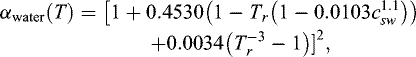 (16)
where csw is the salinity of water, expressed in mol of NaCl per kilogram of solvent.
(16)
where csw is the salinity of water, expressed in mol of NaCl per kilogram of solvent.
It is important to stress that for a given i,j pair, different interaction binary parameters kij can be used for aqueous phase and vapor phase (see Eqs. (11) and (12)), making this approach heterogeneous and thus not suitable to calculate phase equilibrium in the vicinity of critical points. In this section, an aqueous and a vapor interaction binary parameter between hydrogen and salted water is adjusted.
4.2 Binary interaction parameters fitting
The aqueous binary interaction parameter between H2 (i) and salted water (j) adjusted in this work follows the empirical form suggested by Soreide et al. to model CO2 solubility (Soreide and Whitson, 1992):
 (17)
where Ax, αx and βx are empirical adjustable parameters.
(17)
where Ax, αx and βx are empirical adjustable parameters.
Note that this binary interaction parameter is between hydrogen and salted water, since this equation of state does not consider ionic species explicitly. This approach is thus fundamentally different from the molecular simulation one described in Section 3, where the optimized binary parameters (ξij = 0 and lij = −0.24) represent explicitly the interactions between hydrogen and the ions Na+ and Cl−.
These SW empirical parameters are adjusted in order to reproduce experimental Henry constants of hydrogen in pure water up to 573 K (smoothed experimental data by correlation 3 are used), experimental Henry constants of hydrogen in salted water from 273 to 323 K and salinities from 0.5 to 2 mol/kgH2O, and simulated Henry constant obtained from molecular simulation from 273 to 573 K and salinities from 0.5 to 2 mol/kgH2O. The optimized parameters are given in Table 6. The resulting equation of state matches the experimental data with an average deviation of 0.3% for pure water, and 3% for salted water, as shown in Figure 5.
After the calibration of the SW interaction binary parameters for the aqueous phase, the kij in the vapor phase were adjusted to match experimental gaseous composition in binary H2 + H2O system (Gillespie and Wilson, 1980) at given temperatures and pressures, for temperatures ranging from 310 to 440 K and pressures from 3 to 140 bar. The optimized values are given in Table 6 and lead to an average deviation between calculated and experimental data of about 6.5% (Fig. 6).
Optimized interaction binary parameter between H2 and salted water for the aqueous phase and vapor phase of the Soreide and Whitson equation of state.
 |
Fig. 5 Henry constant of H2 in aqueous NaCl solutions versus temperature. Open symbols: experimental data in salted water. Filled symbols: Monte Carlo simulation results (diamonds: NaCl = 0.5 mol/kgH2O, squares: NaCl = 1 mol/kgH2O, triangles: NaCl = 2 mol/kgH2O). Dashed red line: pure water correlation (Eq. (3)). Solid black lines: Calibrated SW equation of state. |
 |
Fig. 6 Experimental data and computed dew curves for the system H2 + H2O. Symbols: experimental data (Gillespie and Wilson, 1980) at 310.93 K (circles), 366.48 K (squares), 422.04 K (triangles) and 477.59 K (diamonds). Solid lines: SW equation of state. |
5 Geological applications
In order to illustrate the possible applications of the thermodynamic work presented in the previous sections, the calibrated SW equation of state was used in several simple calculations relevant for geological situations involving hydrogen.
5.1 Underground storage
The first example concerns hydrogen geological storage. The calibrated Soreide and Whitson equation of state can be used to perform flash calculations to determine both the aqueous and vapor phase compositions. Water content in the produced vapor phase, necessary to design surface facilities, can thus be predicted. Taking as examples hypothetical pure hydrogen storages in the formations of Lobodice, in Czech Republic, and Diadema, in Argentina, and considering the thermodynamic conditions given by Panfilov (2015) (respectively 34 °C/90 bar and 50 °C/10 bar) and seawater salinity for connate waters (0.6 mol/kgH2O NaCl), the developed model predicts water molar fractions in the vapor phase of, respectively, 5.6 × 10⁻⁴ and 1.171 × 10⁻² (Tab. 7). In other words, considering that the two gaseous components and their mixing have similar molar volume, it means that, for each 100 000 m3 of withdrawn gas, a storage in Lobodice would only produce 56 m3 of water vapor versus 1 171 m3 in Diadema. The H2 concentration in the water at equilibrium with these gas phases can also be calculated and would be 0.056 mol/kgH2O in the case of Lobodice and 0.006 mol/kgH2O in the Diadema Formation. As could be expected, pressure is playing a key role on the phase behavior of this system, and can modify by several orders of magnitude the water content in the produced gas.
Thermodynamic conditions considered for the Lobodice and Diadema formations and calculated water molar fractions in the vapor phase and H2 concentrations in the aqueous phase.
5.2 Mid oceanic ridge vents
The geochemistry of the vent fluids around the middle oceanic ridge, especially the Atlantic one that has been studied by various oceanographic campaigns, have all shown high hydrogen concentrations (e.g. Charlou et al., 2002 for the Acores Sea, 36°N). As a second illustrative application case, the phase behavior of native hydrogen in thermodynamic conditions typical of these Mid-Atlantic ridge hydrothermal systems was explored. Hydrothermal fluids temperatures come from (Charlou et al., 2010) and pressures were deduced from the same data-set considering hydrostatic equilibrium. Pure-H2 solubility calculations were performed for temperatures varying between 300 and 350 °C and pressures from 270 to 320 bar with a salinity close to 0.65 mol/kgH2O NaCl. In addition, Lost City (about 30°N on the Atlantic mid oceanic ridge) conditions were also investigated (94 °C and 78 bar), as well as the ones of 3 km-deep seawater (2 °C and 300 bar). The calculated solubilities are indicated in Table 8, and can be compared to the H2 concentrations measured in the corresponding hydrothermal fluid (Charlou et al., 2010). If we consider a negligible effect of the other dissolved gases (measured in lesser concentrations than H2), these hydrothermal systems should be purely monophasic, due to hydrogen content up-to 70 times below the solubility limit. According to these results, the presence of gas bubbles, described by (Charlou et al., 2010) throughout the smokers of Ashadze (mid oceanic ridge, 13°N), is, as mentioned by the authors of this study, “unexpected”. The phase behavior of the H2O-H2-NaCl system alone cannot explain this observation, which should be investigated with a more comprehensive thermodynamic model considering additional species, such as CO2 or H2S.
Thermodynamic conditions considered and calculated H2 solubility in Mid-Atlantic ridge hydrothermal systems. H2 concentrations measured in the corresponding hydrothermal fluids are also indicated.
5.3 Natural continental hydrogen emissions
Natural continental hydrogen emissions have been detected on several geographic locations (Larin et al., 2015; Moretti et al., 2018; Prinzhofer and Deville, 2015; Prinzhofer et al., 2019). In order to investigate the phase behavior of such continental natural emissions, hydrogen solubility was plotted versus depth (Fig. 7). Thermodynamic conditions were estimated considering a surface temperature of 20 °C, a geothermal gradient of 30 °C per km and hydrostatic pressure. Calculations were performed for pure water and brines with salinity of 0.6, 1 and 2 mol/kgH2O NaCl.
Results show that the solubility of hydrogen tends to increase with depth, to rapidly become significant. As an illustration, H2 solubility calculated at 1000 m in pure water (about 0.07 mol/kgH2O) can be compared with the maximum concentration of about 0.01 mol/kgH2O calculated by fluid-rock interactions modeling in Oman ophiolite (Bachaud et al., 2017). This indicates that, in such systems, transport of hydrogen would occur mostly in the aqueous phase and that formation of gaseous H2 would be a quite shallow process.
Due to the salting-out effect, the solubility decreases with increasing salinity, which is observed in Figure 7. The impact of NaCl concentration does not change significantly between 0 and 3000 m: the H2 solubility is about 35% lower in 1 mol/kgH2O NaCl brines than in pure water at each investigated depth, and about 30% lower in 2 mol/kgH2O NaCl solutions than in 1 mol/kgH2O NaCl ones.
Solubility of hydrogen was also compared with the one of methane. Solubility of both components was calculated for depths from 0 to 1500 m considering a salinity of 0.1 mol/kgH2O NaCl. The model parameters for the H2O + CH4 + NaCl system come from the original work of Soreide and Whitson (Soreide and Whitson, 1992). Results are plotted in Figure 8.
The solubility of methane is superior to the hydrogen one down to 1300 m and, below that point, H2 is actually more soluble than CH4. This result can be put in perspective to some observations presented by Prinzhofer et al. (2018) on the hydrogen and methane accumulations discovered in the Bourabougou field (Mali). Indeed, it seems that highest methane contents in the gas phase are found below 1500 m. If a solubility effect alone cannot explain the gas reservoirs organization, the results presented on Figure 8 indicate that a given-composition gas mixture of CH4 and H2 equilibrated with formation water would tend to contain more H2 than CH4 above 1300 m, and more CH4 than H2 below.
 |
Fig. 7 Hydrogen solubility versus depth for NaCl concentrations of 0, 0.6, 1 and 2 mol/kgH2O. |
 |
Fig. 8 Hydrogen and methane solubility versus depth for NaCl concentrations of 0.1 mol/kgH2O. |
6 Conclusion
In this work, Monte Carlo simulations have been carried out to generate new simulated data of hydrogen solubility in aqueous NaCl solutions in temperature and salinity ranges of interest for geological applications, and for which no experimental data are currently available. In order to validate the force field used, a review of existing data for the binary system H2 + H2O and the ternary system H2 + H2O + NaCl is first proposed, all the data being converted into Henry constants. For the simulations, the molecular models of Darkrim for hydrogen (Darkrim et al., 1999), TIP4P/2005 for water (Abascal and Vega, 2005) and OPLS for Na+ and Cl− (Chandrasekhar et al., 1984) have been selected since they are able to accurately reproduce phase property of pure components and brine densities. To model solvent-solutes and solutes-solutes interactions, it was shown that the Lorentz-Berthelot combining rule is the most appropriate to reproduce the experimental hydrogen Henry constants. Nevertheless, it was necessary to correct the cross-diameter of the Lorentz-Berthelot combining rule between H2 and Na+ and Cl− with a constant binary interaction parameter. With this force field, simulation results reproduce the hydrogen Henry constant in salted water with an average deviation of 6%. Simulation results accurately predict the expected behavior such as the salting-out effect and the maximum of hydrogen solubility close to 330 K. This force field was then used in extrapolation to generate Henry constant for temperatures up to 573 K and salinities up to 2 mol/kgH2O. It is worth noticing that the extrapolation at higher salinities is questionable, and adding additional molecular interactions in the force field, such as polarization, could be useful to keep the predictivity of the approach. Using the experimental data and these new simulated data generated by molecular simulation at higher temperatures and salinities, a binary interaction parameter of the Soreide and Whitson equation of state has been fitted in order to extend the validity range of this thermodynamic model for systems containing hydrogen and salted water. This new parameterization of the equation of state allows a fast and reliable calculations of phase equilibrium for the H2 + H2O + NaCl system in a range of temperatures and salinities corresponding to subsurface conditions. Consequently, this model allows to predict hydrogen phase behavior in various geological contexts. To illustrate the possible use of the model, simple situations involving hydrogen in subsurface were investigated. In particular, the results showed that:
-
at low depths (typically below 200 m) hydrogen solubility is low, suggesting that, close to the surface, transportation through the aqueous phase should only lead to minor hydrogen migrations;
-
in underground storages (for which temperature is usually lower than 60 °C), the key factor governing the phase equilibrium is the pressure rather than salinity;
-
when temperature and pressure increase, such as in the hydrothermal vents or at important depths, a larger amount of hydrogen can be dissolved in water (typically around 100 times more at a depth of 1000 meter than in surface conditions), indicating that deep aquifers or hydrothermal fluids could be a major transport mode for hydrogen.
Acknowledgments
Authors gratefully acknowledge Dr. J.C. de Hemptinne and Dr. E. Brosse (IFPEN) for fruitful discussions. This work is extracted from the Master Thesis of Cristina Lopez Lazaro which has been funded by ENGIE.
References
- Abascal JLF, Vega C. 2005. A general purpose model for the condensed phases of water: TIP4P/2005. J Chem Phys 123(23): 234505. [CrossRef] [PubMed] [Google Scholar]
- ADEME. 2018. Methycentre – Unité de Power-to-Gas couplée à une unité de méthanisation. Available from https://www.ademe.fr/methycentre. [Google Scholar]
- Ahmed S, Ferrando N, Hemptinne J-C de, Simonin J-P, Bernard O, Baudouin O. 2016. A new PC-SAFT model for pure water, water–hydrocarbons, and water–oxygenates systems and subsequent modeling of VLE, VLLE, and LLE. J Chem Eng Data 61(12): 4178–4190. [CrossRef] [Google Scholar]
- Ahmed S, Ferrando N, Hemptinne J-C de, Simonin J-P, Bernard O, Baudouin O. 2018. Modeling of mixed-solvent electrolyte systems. Fluid Phase Equilib 459: 138–157. [CrossRef] [Google Scholar]
- Ahrens M, Heusler KE. 1981. Solubilities of some gases in liquid ammonia. Z Phys Chem NF 1981: 127–128. [CrossRef] [Google Scholar]
- Akinfiev NN, Diamond LW. 2003. Thermodynamic description of aqueous nonelectrolytes at infinite dilution over a wide range of state parameters. Geochim Cosmochim Acta 67(4): 613–629. [CrossRef] [Google Scholar]
- Allen MP, Tildesley DJ. 1987. Computer simulation of liquids. Oxford: University Press. [Google Scholar]
- Alvarez J, Crovetto R, Fernandez-Prini R. 1988. The dissolution of N2 and of H2 in water from room temperature to 640 K. Ber Bunsen-Ges Phys Chem 92: 935–940. [CrossRef] [Google Scholar]
- Bachaud P, Meiller C, Brosse E, Durand I, Beaumont V. 2017. Modeling of hydrogen genesis in ophiolite massif. Proced Earth Plan Sc 17: 265–268. [CrossRef] [Google Scholar]
- Bohr C. 1905. Absorptionscoëfficienten des Blutes und des Blutplasmas für Gase 1. Skandinavisches Archiv Für Physiologie 17(1): 104–112. [CrossRef] [Google Scholar]
- Braun L. 1900. Solubility Data Series. Z Phys Chem 33: 721–741. [Google Scholar]
- Bunsen R. 1855. On the law of absorption of gases. Philos Mag J Sci 9: 116–130. [CrossRef] [Google Scholar]
- Carden P, Paterson L. 1979. Physical, chemical and energy aspects of underground hydrogen storage. Int J Hydrogen Energy 4(6): 559–569. [CrossRef] [Google Scholar]
- Carvalho PJ, Pereira LMC, Gonçalves NPF, Queimada AJ, Coutinho JAP. 2015. Carbon dioxide solubility in aqueous solutions of NaCl. Measurements and modeling with electrolyte equations of state. Fluid Phase Equilib 388: 100–106. [CrossRef] [Google Scholar]
- Cassuto L. 1903. Sulla solubilità dei gas nei liqdidi. Il Nuovo Cimento (1901-1910) 6(1): 5–20. [CrossRef] [Google Scholar]
- Chandrasekhar J, Spellmeyer DC, Jorgensen WL. 1984. Energy component analysis for dilute aqueous solutions of lithium(1+), sodium(1+), fluoride(1−), and chloride(1−) ions. J Am Chem Soc 106(4): 903–910. [CrossRef] [Google Scholar]
- Charlou JL, Donval JP, Fouquet Y, Jean-Baptiste P, Holm N. 2002. Geochemistry of high H2 and CH4 vent fluids issuing from ultramafic rocks at the Rainbow hydrothermal field (36°14′N, MAR). Chemical Geology 191(4): 345–359. [CrossRef] [Google Scholar]
- Charlou J-L, Donval JP, Konn C, Ondreas H, Fouquet Y, Jean-Baptiste P, et al. 2010. High production and fluxes of H2 and CH4 and evidence of abiotic hydrocarbon synthesis by serpentinization in ultramafic-hosted hydrothermal systems on the Mid-Atlantic Ridge. Washington DC American Geophysical Union Geophysical Monograph Series 188: 265–295. [Google Scholar]
- Choudhary VR, Parande MG, Brahme PH. 1982. Simple apparatus for measuring solubility of gases at high pressures. Ind Eng Chem Fund 21(4): 472–474. [CrossRef] [Google Scholar]
- Courtial X, Ferrando N, Hemptinne J-C de, Mougin P. 2014. Electrolyte CPA equation of state for very high temperature and pressure reservoir and basin applications. Geochim Cosmochim Acta 142(Supplement C): 1–14. [CrossRef] [Google Scholar]
- Cramer SD. 1982. The solubility of methane, carbon dioxide, and oxygen in brines from 0 degrees to 300 °C. Bur Mines Rep Invest RI 8706: 1–17. [Google Scholar]
- Creton B, Nieto-Draghi C, Bruin T de, Lachet V, El Ahmar E, Valtz A, et al. 2018. Thermodynamic study of binary systems containing sulphur dioxide and nitric oxide. Measurements and modelling. Fluid Phase Equilib 461: 84–100. [CrossRef] [Google Scholar]
- Crozier TE, Yamamoto S. 1974. Solubility of hydrogen in water, sea water, and sodium chloride solutions. J Chem Eng Data 19(3): 242–244. [CrossRef] [Google Scholar]
- Darkrim F, Vermesse J, Malbrunot P, Levesque D. 1999. Monte Carlo simulations of nitrogen and hydrogen physisorption at high pressures and room temperature. Comparison with experiments. J Chem Phys 110(8): 4020–4027. [CrossRef] [Google Scholar]
- Darras C, Muselli M, Poggi P, Voyant C, Hoguet J-C, Montignac F. 2012. PV output power fluctuations smoothing. The MYRTE platform experience. Int J Hydrogen Energy 37(19): 14015–14025. [CrossRef] [Google Scholar]
- Delhommelle J, Millie P. 2001. Inadequacy of the Lorentz-Berthelot combining rules for accurate predictions of equilibrium properties by molecular simulation. Mol Phys 99: 619–625. [CrossRef] [Google Scholar]
- Deville E, Prinzhofer A. 2016. The origin of N2-H2-CH4-rich natural gas seepages in ophiolitic context: A major and noble gases study of fluid seepages in New Caledonia. Chem Geol 440: 139–147. [CrossRef] [Google Scholar]
- Dohrn R, Brunner G. 1986. Phase equilibria in ternary and quaternary systems of hydrogen, water and hydrocarbons at elevated temperatures and pressures. Fluid Phase Equilib 29: 535–544. [CrossRef] [Google Scholar]
- Drucker K, Moles E. 1910. Gas solubility in aqueous solutions of glycerol and isobutyric acid. Z Phys Chem Stoechiom Verwandtschaftsl 75: 405–436. [Google Scholar]
- Duan ZH, Sun R. 2003. An improved model calculating CO2 solubility in pure water and aqueous NaCl solutions from 273 to 533 K and from 0 to 2000 bar. Chem Geol 193(3–4): 257–271. [CrossRef] [Google Scholar]
- Duan Z, Moller N, Weare JH. 1996. Prediction of the solubility of H2S in NaCl aqueous solution: An equation of state approach. Chem Geol 130: 15–20. [CrossRef] [Google Scholar]
- Duan Z, Moller N, Weare JH. 2003. Equations of state for the NaCl-H2O-CH4 system and the NaCl-H2O-CO2-CH4 system: Phase equilibria and volumetric properties above 573 K. Geochim Cosmochim Acta 67: 671–680. [CrossRef] [Google Scholar]
- Duan ZH, Moller N, Greenberg J, Weare JH. 1992. The prediction of methane solubility in natural-waters to high ionic-strength from 0-degrees-C to 250-degrees-C and from 0 to 1600 Bar. Geochim Cosmochim Acta 56(4): 1451–1460. [CrossRef] [Google Scholar]
- ENGIE. 2018. GRHYD. Available from https://www.engie.com/innovation-transition-energetique/pilotage-digital-efficacite-energetique/power-to-gas/projet-demonstration-grhyd/. [Google Scholar]
- Fauve R, Guichet X, Lachet V, Ferrando N. 2017. Prediction of H2S solubility in aqueous NaCl solutions by molecular simulation. J Pet Sci Eng 157: 94–106. [CrossRef] [Google Scholar]
- Fernández-Prini R, Alvarez JL, Harvey AH. 2003. Henry’s constants and vapor-liquid distribution constants for gaseous solutes in H2O and D2O at high temperatures. J Phys Chem Ref Data 32(2): 903–916. [CrossRef] [Google Scholar]
- Ferrando N, Ungerer P. 2007. Hydrogen/hydrocarbon phase equilibrium modelling with a cubic equation of state and a Monte Carlo method. Fluid Phase Equilib 254(1–2): 211–223. [CrossRef] [Google Scholar]
- Findlay A, Shen B. 1912. The influence of colloids and fine suspensions on the solubility of gases in water. Part II. Solubility of carbon dioxide and hydrogen. J Chem Soc 101: 1459–1468. [CrossRef] [Google Scholar]
- Frenkel D, Smit B. 1996. Understanding molecular simulation: From algorithms to applications. San Diego: Academic Press. [Google Scholar]
- Gamsjäger H, Lorimer JW, Salomon M, Shaw DG, Tomkins RPT. 2010. The IUPAC-NIST solubility data series: A guide to preparation and use of compilations and evaluations. J Phys Chem Ref Data 39(2): 23101. [CrossRef] [Google Scholar]
- Geffken G. 1904. Contribution on the knowledge of the interference solubility. Z Phys Chem Stoechiom Verwandtschaftsl 49: 257–302. [Google Scholar]
- Gerecke J, Bittrich HJ. 1971. The solubility of H2, CO2 and NH3 in an aqueous electrolyte solution. Wiss Z Tech Hochsch Chem Carl Shorlemmer Leuna Merseburg 13: 115–122. [Google Scholar]
- Gillespie PC, Wilson GM. 1980. Vapor-liquid equilibrium data on water-substitute gas components: N2-H2O, H2-H2O, CO-H2O, H2-CO-H2O and H2S-H2O. GPA Research Report, 1980. [Google Scholar]
- Gniewosz S, Walfisz A. 1887. The absorption of gases by petroleum. Z Phys Chem Stoechiom Verwandtschaftsl 1: 70–72. [Google Scholar]
- Gordon LI, Cohen Y, Standley DR. 1977. The solubility of molecular hydrogen in seawater. Deep Sea Research 24(10): 937–941. [CrossRef] [Google Scholar]
- Guélard J, Beaumont V, Rouchon V, Guyot F, Pillot D, Jézéquel D, et al. 2017. Natural H2 in Kansas. Deep or shallow origin? Geochem Geophys Geosyst 18(5): 1841–1865. [CrossRef] [Google Scholar]
- Held C, Reschke T, Mohammad S, Luza A, Sadowski G. 2014. ePC-SAFT revised. Chem Eng Res Des 92(12): 1884–1897. [CrossRef] [Google Scholar]
- Hemptinne JC de, Mougin P, Barreau A, Ruffine L, Tamouza S, Inchekel R. 2006. Application to petroleum engineering of statistical thermodynamics– Based equations of state. Oil & Gas Sci Tech – Rev IFP Energies nouvelles 61(3): 363–386. [CrossRef] [Google Scholar]
- Huefner G. 1907. Study of the absorption of nitrogen and hydrogen in aqueous solutions. Z Phys Chem Stoechiom Verwandtschaftsl 57: 611–625. [Google Scholar]
- Ipatev VV, Druzhina-Artemovitch SI, Tikhomirov VI. 1931. Solubility of hydrogen in water under pressure. Zh Obshch Khim 1: 594–597. [Google Scholar]
- Ipatiew WW, Drushina-Artemowitsch SI, Tichomirow WI. 1932. Löslichkeit des Wasserstoffs in Wasser unter Druck. Ber dtsch Chem Ges A/B 65 (4): 568–571. [CrossRef] [Google Scholar]
- Ji X, Tan SP, Adidharma H, Radosz M. 2005. SAFT1-RPM approximation extended to phase equilibria and densities of CO2-H2O and CO2-H2O-NaCl systems. Ind Eng Chem Res 44(22): 8419–8427. [CrossRef] [Google Scholar]
- Jiang H, Economou IG, Panagiotopoulos AZ. 2017. Molecular modeling of thermodynamic and transport properties for CO2 and aqueous brines. Acc Chem Res 50(4): 751–758. [CrossRef] [Google Scholar]
- Kishima N, Sakai H. 1984. Fugacity-concentration relationship of dilute hydrogen in water at elevated temperature and pressure. Earth Planet Sci Lett 67(1): 79–86. [CrossRef] [Google Scholar]
- Knaster MB, Apelbaum LA. 1964. Solubility of hydrogen and oxygen in concentrated potassium hydroxide solution. Russ J Phys Chem 38: 120–122. [Google Scholar]
- Kong CL. 1973. Combining rules for intermolecular potential parameters. II. Rules for the Lennard-Jones (12-6) potential and the Morse potential. J Chem Phys 59: 2464. [CrossRef] [Google Scholar]
- Kontogeorgis GM, Folas GK. 2010. Thermodynamic models for industrial applications: From classical and advanced mixing rules to association theories. Chichester: Wiley. [Google Scholar]
- Larin N, Zgonnik V, Rodina S, Deville E, Prinzhofer A, Larin VN. 2015. Natural molecular hydrogen seepage associated with surficial, rounded depressions on the European Craton in Russia. Natural Resources Research 24(3): 369–383. [CrossRef] [Google Scholar]
- Le Duigou A, Bader A-G., Lanoix J-C., Nadau L. 2017. Relevance and costs of large scale underground hydrogen storage in France. Int J Hydrogen Energy 42(36): 22987–3003. [CrossRef] [Google Scholar]
- Li D, Beyer C, Bauer S. 2018. A unified phase equilibrium model for hydrogen solubility and solution density. Int J Hydrogen Energy 43(1): 512–529. [CrossRef] [Google Scholar]
- Li J, Wei L, Li X. 2015. An improved cubic model for the mutual solubilities of CO2-CH4-H2S-brine systems to high temperature, pressure and salinity. Applied Geochemistry 54: 1–12. [CrossRef] [Google Scholar]
- Liu Y, Lafitte T, Panagiotopoulos AZ, Debenedetti PG. 2013. Simulations of vapor-liquid phase equilibrium and interfacial tension in the CO2-H2O-NaCl system. AIChE J 59(9): 3514–3522. https://doi.org/10.1002/aic.14042. [CrossRef] [Google Scholar]
- Llovell F, Marcos RM, MacDowell N, Vega LF. 2012. Modeling the absorption of weak electrolytes and acid gases with ionic liquids using the soft-SAFT approach. J Phys Chem B 116(26): 7709–7718. [CrossRef] [Google Scholar]
- Longo LD, Delivora-Papadopoulos M, Power GG, Hill EP, Forster RE. 1970. Diffusion equilibration of inert gases between maternal and fetal placenta capillaries. Am J Physiol 1970: 561–569. [CrossRef] [Google Scholar]
- Lord AS, Kobos PH, Borns DJ. 2014. Geologic storage of hydrogen. Scaling up to meet city transportation demands. Int J Hydrogen Energy 39(28): 15570–15582. [CrossRef] [Google Scholar]
- Lubarsch O. 1889. Ueber die Absorption von Gasen in Gemischen von Alkohol und Wasser. Ann Phys 273(7): 524–525. [CrossRef] [Google Scholar]
- Mackie AD, Tavitian B, Boutin A, Fuchs AH. 1997. Vapour-liquid phase equilibria predictions of methane-alkane mixtures by Monte Carlo simulation. Mol Sim 19(1): 1–15. [CrossRef] [Google Scholar]
- Maribo-Mogensen B, Thomsen K, Kontogeorgis GM. 2015. An electrolyte CPA equation of state for mixed solvent electrolytes. AIChE J 61(9): 2933–2950. [CrossRef] [Google Scholar]
- Meyer M, Tebbe U, Piiper J. 1980. Solubility of inert gases in dog blood and skeletal muscle. Pflügers Archiv 384(2): 131–134. [CrossRef] [Google Scholar]
- Milligan LH. 1923. The solubility of gasoline (hexane and heptane) in water at 25 °C. J Phys Chem 28(5): 494–497. https://doi.org/10.1021/j150239a006. [CrossRef] [Google Scholar]
- Moretti I, Dagostino A, Werly J, Ghost C, Defrenne D, Gorintin L. 2018. L’hydrogène naturel : un nouveau pétrole ? Pour la Science 485: 22–26. [Google Scholar]
- Morris DR, Yang L, Giraudeau F, Sun X, Steward FR. 2001. Henry’s law constant for hydrogen in natural water and deuterium in heavy water. Phys Chem Chem Phys 3(6): 1043–1046. [CrossRef] [Google Scholar]
- Morrison TJ, Billett F. 1952. 730. The salting-out of non-electrolytes. Part II. The effect of variation in non-electrolyte. J Chem Soc (0): 3819–3822. https://doi.org/10.1039/JR9520003819. [CrossRef] [Google Scholar]
- Mueller C. 1912. The absorption of oxygen, nitrogen and hydrogen in aqueous solution of non-electrolytes. Z Phys Chem Stoechiom Verwandtschaftsl 81: 483–503. [Google Scholar]
- Nezbeda I, Kolafa J. 1991. A new version of the insertion particle method for determining the chemical potential by Monte Carlo simulation. Mol Sim 5: 391–403. [CrossRef] [Google Scholar]
- Nichita DV, Broseta D, Elhorga P, Montel F. 2008. Pseudo-component delumping for multiphase equilibrium in hydrocarbon-water mixtures. Petroleum Science and Technology 26(17): 2058–2077. [CrossRef] [Google Scholar]
- Panfilov M. 2015. Underground and pipeline hydrogen storage. In Subramani V, Basile A, Veziroğlu TN, eds.Compendium of hydrogen energy. Cambridge, UK: Woodhead Publishing, an imprint of Elsevier, pp. 91–115. [Google Scholar]
- Patel BH, Paricaud P, Galindo A, Maitland GC. 2003. Prediction of the salting-out effect of strong electrolytes on water + alkane solutions. Ind Eng Chem Res 42(16): 3809–3823. [CrossRef] [Google Scholar]
- Paterson L. 1983. The implications of fingering in underground hydrogen storage. Int J Hydrogen Energy 8(1): 53–59. [CrossRef] [Google Scholar]
- Peng DY, Robinson DB. 1976. A new two-constant equation of state. Ind Eng Chem Fund 15(1): 59–64. [Google Scholar]
- Perez A, Perez E, Dupraz S, Bolcich J. 2016. 21st World Hydrogen Energy Conference 2016 (WHEC 2016), Zaragossa, Spain, 2016. [Google Scholar]
- Plennevaux C, Ferrando N, Kittel J, Frégonèse M, Normand B, Cassagne T, et al. 2013. pH prediction in concentrated aqueous solutions under high pressure of acid gases and high temperature. Corros Sci 73: 143–149. [CrossRef] [Google Scholar]
- Plyasunov AV, Bazarkina EF. 2018. Thermodynamic properties of dilute hydrogen in supercritical water. Fluid Phase Equilib 470: 140–148. [CrossRef] [Google Scholar]
- Plyasunov AV, Shock EL. 2001. Correlation strategy for determining the parameters of the revised Helgeson-Kirkham-Flowers model for aqueous nonelectrolytes. Geochim Cosmochim Acta 65(21): 3879–3900. [CrossRef] [Google Scholar]
- Power GG, Stegall H. 1970. Solubility of gases in human red blood cell ghosts. J Appl Physiol 29: 145–149. [CrossRef] [Google Scholar]
- Pray HA, Schweickert CE, Minnich BH. 1952. Solubility of hydrogen, oxygen, nitrogen, and helium in water at elevated temperatures. Ind Eng Chem 44(5): 1146–1151. [CrossRef] [Google Scholar]
- Prinzhofer A, Deville E. 2015. Hydrogène naturel. La prochaine révolution énergétique ? Paris : Belin. [Google Scholar]
- Prinzhofer A, Cisse CST, Diallo AB. 2018. Discovery of a large accumulation of natural hydrogen in Bourakebougou (Mali). Int J Hydrogen Energy 43: 19315–19326. [Google Scholar]
- Prinzhofer A, Moretti I, Françolin J, Pacheco C, D’Agostino A, Werly J, et al. 2019. Natural hydrogen continuous emission from sedimentary basins. The example of a Brazilian H2-emitting structure. Int J Hydrogen Energy 44(12): 5676–5685. [Google Scholar]
- Purwanto, Deshpande RM, Chaudhari RV, Delmas H. 1996. Solubility of hydrogen, carbon monoxide, and 1-octene in various solvents and solvent mixtures. J Chem Eng Data 41(6): 1414–1417. [CrossRef] [Google Scholar]
- Qiao C, Li L, Johns RT, Xu J. 2016. Compositional modeling of dissolution-induced injectivity alteration during CO2 flooding in carbonate reservoirs. SPE J 21(3): 809–826. [CrossRef] [Google Scholar]
- Reitenbach V, Ganzer L, Albrecht D, Hagemann B. 2015. Influence of added hydrogen on underground gas storage: A review of key issues. Environ. Earth Sci 73(11): 6927–6937. [CrossRef] [Google Scholar]
- Rowe AM. 1970. Pressure- volume-temperature concentration relation of aqueous NaCl solutions. J Chem Eng Data 15(1): 61–66. [CrossRef] [Google Scholar]
- Rowley RL, Wilding WV, Oscarson JL, Yang Y, Zundel NA, Daubert TE, et al. 2003. DIPPR® data compilation of pure compounds properties. New York, NY: Design Institute for Physical Properties, AIChE. [Google Scholar]
- Rozmus J, Hemptinne JC de, Galindo A, Dufal S, Mougin P. 2013. Modeling of strong electrolytes with ePPC-SAFT up to high temperatures. Ind Eng Chem Res 52: 9979–9994. [CrossRef] [Google Scholar]
- Ruetschi P, Amlie RF. 1966. Solubility of hydrogen in potassium hydroxide and sulfuric acid. Salting-out and hydration. J Phys Chem 70(3): 718–723. [CrossRef] [Google Scholar]
- Rumpf B, Xia J, Maurer G. 1998. Solubility of carbon dioxide in aqueous solutions containing acetic acid or sodium hydroxide in the temperature range from 313 to 433 K and at total pressures up to 10 MPa. Ind Eng Chem Res 37(5): 2012–2019. [CrossRef] [Google Scholar]
- Satake H, Ohashi M, Hayashi Y. 1984. Discharge of H2 from the Atotsugawa and Ushikubi Faults, Japan, and its relation to earthquakes. Pure and Applied Geophysics 122(2): 185–193. [CrossRef] [Google Scholar]
- Sato M, Sutton AJ, McGee KA, Russell-Robinson S. 1986. Monitoring of hydrogen along the San Andreas and Calaveras faults in central California in 1980- 1984. J Geophys Res 91(B12): 12315–12326. [CrossRef] [Google Scholar]
- Seward TM, Franck EU. 1981. The system hydrogen – water up to 440 °C and 2500 bar pressure. Berichte der Bunsen-Gesellschaft-Physical Chemistry Chemical Physics 85(1): 2–7. [CrossRef] [Google Scholar]
- Soave G. 1972. Equilibrium constants for a modified Redlich-Kwong equation of state. Chem Eng Sci 27: 1197–1203. [Google Scholar]
- Soreide I, Whitson C. 1992. Peng-Robinson predictions for hydrocarbons, CO2, N2, and H2S with pure water and NaCl brine. Fluid Phase Equilib 77: 217–240. [CrossRef] [Google Scholar]
- Sorensen H, Pedersen KS, Christensen PL. 2002. Modeling of gas solubility in brines. Org Geochem 33: 635–642. [CrossRef] [Google Scholar]
- Stefánsson A, Seward TM. 2003. Stability of chloridogold(I) complexes in aqueous solutions from 300 to 600 °C and from 500 to 1800 bar. Geochim Cosmochim Acta 67(23): 4559–4576. [CrossRef] [Google Scholar]
- Steiner P. 1894. Über die Absoprtion des Wasserstoffs im Wasser und in wässerigen Lösungen. Annalen der Physik und Chemie 52: 275–299. [CrossRef] [Google Scholar]
- Sun R, Dubessy J. 2012. Prediction of vapor-liquid equilibrium and PVTx properties of geological fluid system with SAFT-LJ EOS including multi-polar contribution. Part II: Application to H2O-NaCl and CO2 + H2O + NaCl System. Geochim Cosmochim Acta 88(0): 130–145. [CrossRef] [Google Scholar]
- Theodorou DN. 2010. Progress and outlook in Monte Carlo simulations. Ind Eng Chem Res 49: 3047–3058. [CrossRef] [Google Scholar]
- Timofeev VS. 1890. The absorption of hydrogen and oxygen in water and alcohol. Z Phys Chem Stoechiom Verwandtschaftsl 6: 141–152. [Google Scholar]
- Torrie GM, Valleau JP. 1977. Non-physical sampling distributions in Monte-Carlo free-energy estimation – Umbrella Sampling. J Comput Phys 23(2): 187–199. [NASA ADS] [CrossRef] [Google Scholar]
- Trinh T-K-H, Hemptinne J-C de, Lugo R, Ferrando N, Passarello J-P. 2016a. Hydrogen solubility in hydrocarbon and oxygenated organic compounds. J Chem Eng Data 61(1): 19–34. https://doi.org/10.1021/acs.jced.5b00119. [CrossRef] [Google Scholar]
- Trinh T-K-H, Passarello J-P, Hemptinne J-C de, Lugo R, Lachet V. 2016b. A non-additive repulsive contribution in an equation of state: The development for homonuclear square well chains equation of state validated against Monte Carlo simulation. J Chem Phys 144(12): 124902. Available from http://scitation.aip.org/content/aip/journal/jcp/144/12/10.1063/1.4944068. [CrossRef] [Google Scholar]
- Tsai ES, Jiang H, Panagiotopoulos AZ. 2016. Monte Carlo simulations of H2O-CaCl2 and H2O-CaCl2-CO2 mixtures. Fluid Phase Equilib 407: 262–268. [CrossRef] [Google Scholar]
- Ungerer P, Tavitian B, Boutin A. 2005. Applications of molecular simulation in the oil and gas industry. Paris: Editions Technip. [Google Scholar]
- Ungerer P, Wender A, Demoulin G, Bourasseau E, Mougin P. 2004. Application of Gibbs ensemble and NPT Monte Carlo simulation to the development of improved processes for H2S-rich Gases. Mol Sim 30(10): 631–648. [CrossRef] [Google Scholar]
- Vacquand C, Deville E, Beaumont V, Guyot F, Sissmann O, Pillot D, et al. 2018. Reduced gas seepages in ophiolitic complexes. Evidences for multiple origins of the H2-CH4-N2 gas mixtures. Geochim Cosmochim Acta 223: 437–461. [CrossRef] [Google Scholar]
- Vorholz J, Harismiadis VI, Panagiotopoulos AZ, Rumpf B, Maurer G. 2004. Molecular simulation of the solubility of carbon dioxide in aqueous solutions of sodium chloride. Fluid Phase Equilib 226: 237–250. [CrossRef] [Google Scholar]
- Waldmann M, Hagler AT. 1993. New combining rules for rare gas van der waals parameters. J Comput Chem 14: 1077–1084. [CrossRef] [Google Scholar]
- Wei Z, Zhang D. 2013. A fully coupled multiphase multicomponent flow and geomechanics model for enhanced coalbed-methane recovery and CO2 storage. SPE J 18(3): 448–467. [CrossRef] [Google Scholar]
- Wet WJ de. 1964. Determination of gas solubilities in water and some organc liquids. J S Afr Chem Inst 17: 9–13. [Google Scholar]
- Widom B. 1963. Some topics in the theory of fluids. J Chem Phys 39: 2808–2812. [CrossRef] [Google Scholar]
- Winkler LW. 1891. Die Löslichkeit der Gase in Wasser. Ber Dtsch Chem Ges 24(1): 89–101. [CrossRef] [Google Scholar]
- Winkler LW. 1906. Regularity in the absorption of gases in liquids (second communication). Z Phys Chem Stoechiom Verwandtschaftsl 55: 344–354. [Google Scholar]
- Xia J, Rumpf B, Maurer G. 1999. Solubility of carbon dioxide in aqueous solutions containing sodium acetate or ammonium acetate at temperatures from 313 to 433 K and pressures up to 10 MPa. Fluid Phase Equilib 155(1): 107–125. [CrossRef] [Google Scholar]
- Xia J, Pérez-Salado Kamps Á, Rumpf B, Maurer G. 2000. Solubility of hydrogen sulfide in aqueous solutions of the single salts sodium sulfate, ammonium sulfate, sodium chloride, and ammonium chloride at temperatures from 313 to 393 K and total pressures up to 10 MPa. Ind Eng Chem Res. 39(4): 1064–1073. https://doi.org/10.1021/ie990416p. [CrossRef] [Google Scholar]
- Yan W, Huang S, Stenby EH. 2011. Measurement and modeling of CO2 solubility in NaCl brine and CO2-saturated NaCl brine density. International Journal of Greenhouse Gas Control 5(6): 1460–1477. [CrossRef] [Google Scholar]
- Younglove BA. 1982. Thermophysical properties of fluids I. Argon, ethylene, parahydrogen, nitrogen, nitrogen trifluoride and oxygen. J Phys Chem Ref Data 11(Supplement 1): 1. [CrossRef] [Google Scholar]
Cite this article as: Lopez-Lazaro C, Bachaud P, Moretti I, Ferrando N. 2019. Predicting the phase behavior of hydrogen in NaCl brines by molecular simulation for geological applications, BSGF - Earth Sciences Bulletin 190: 7.
All Tables
Optimized interaction binary parameters for the modified Lorentz-Berthelot combining rule.
Optimized interaction binary parameter between H2 and salted water for the aqueous phase and vapor phase of the Soreide and Whitson equation of state.
Thermodynamic conditions considered for the Lobodice and Diadema formations and calculated water molar fractions in the vapor phase and H2 concentrations in the aqueous phase.
Thermodynamic conditions considered and calculated H2 solubility in Mid-Atlantic ridge hydrothermal systems. H2 concentrations measured in the corresponding hydrothermal fluids are also indicated.
All Figures
|
Fig. 1 Compilation of data: Henry constant of H2 in pure water versus temperature. Symbols: experimental data (circles: from Bunsen coefficients, diamonds: Henry constants, triangles: from TPx data, crosses: from Kuenen coefficients, stars: from Ostwald coefficients). Solid line: correlation (Eq. (3)). Dotted lines: uncertainty domain (±10% from the correlation). |
| In the text | |
|
Fig. 2 Experimental and computed Henry constant of H2 in aqueous NaCl solutions versus temperature. Open symbols: experimental data. Filled symbols: simulation results with modified Lorentz-Berthelot combining rule and lij = 0.24 (diamonds: NaCl = 0.5 mol/kgH2O, squares: NaCl = 1 mol/kgH2O, triangles: NaCl = 2 mol/kgH2O). |
| In the text | |
|
Fig. 3 Experimental and computed Henry constant of H2 in pure water versus temperature. Solid line: correlation of experimental data. Dashed lines: experimental uncertainty domain (±10%). Symbols: simulation results with different combining rules (diamonds: Lorentz-Berthelot, squares: Kong, triangles: Waldmann-Hagler). |
| In the text | |
|
Fig. 4 Experimental and computed Henry constant of H2 in aqueous NaCl solutions versus temperature. Open symbols: experimental data. Filled symbols: simulation results with unmodified Lorentz-Berthelot combining rules (squares: NaCl = 1 mol/kgH2O, triangles: NaCl = 2 mol/kgH2O). |
| In the text | |
|
Fig. 5 Henry constant of H2 in aqueous NaCl solutions versus temperature. Open symbols: experimental data in salted water. Filled symbols: Monte Carlo simulation results (diamonds: NaCl = 0.5 mol/kgH2O, squares: NaCl = 1 mol/kgH2O, triangles: NaCl = 2 mol/kgH2O). Dashed red line: pure water correlation (Eq. (3)). Solid black lines: Calibrated SW equation of state. |
| In the text | |
|
Fig. 6 Experimental data and computed dew curves for the system H2 + H2O. Symbols: experimental data (Gillespie and Wilson, 1980) at 310.93 K (circles), 366.48 K (squares), 422.04 K (triangles) and 477.59 K (diamonds). Solid lines: SW equation of state. |
| In the text | |
|
Fig. 7 Hydrogen solubility versus depth for NaCl concentrations of 0, 0.6, 1 and 2 mol/kgH2O. |
| In the text | |
|
Fig. 8 Hydrogen and methane solubility versus depth for NaCl concentrations of 0.1 mol/kgH2O. |
| In the text | |
Current usage metrics show cumulative count of Article Views (full-text article views including HTML views, PDF and ePub downloads, according to the available data) and Abstracts Views on Vision4Press platform.
Data correspond to usage on the plateform after 2015. The current usage metrics is available 48-96 hours after online publication and is updated daily on week days.
Initial download of the metrics may take a while.